from sklearn.model_selection import train_test_split, cross_validate, cross_val_predict, \
                                    StratifiedKFold, KFold
import pandas as pd
from xgboost import XGBClassifier
from sklearn.metrics import ConfusionMatrixDisplay, confusion_matrix, classification_report
import matplotlib.pyplot as plt30 K-fold validation (Titanic Dataset)
We have mentioned k-fold validation a few times throughout the exercises.
We split data into a number of ‘folds’ - let’s say 10. This means we have 10 datasets, each with 10% of the data from our whole* dataset in.
We use 90% of the data to train on, and 10% as our validation dataset.
We record this score, then use a different 10% to score our model on, training our model on the remaining 90%.
We repeat this until every ‘fold’ has been used as the validation dataset once.
Note: Here, we apply k-fold validation after splitting out a final testing dataset to use later.
K-fold validation replaces the train/validate data split.
There are various helper functions within sklearn to allow us to undertake k-fold validation.
try:
    data = pd.read_csv("data/processed_data.csv")

except FileNotFoundError:
    # Download processed data:
    address = 'https://raw.githubusercontent.com/MichaelAllen1966/' + \
                '1804_python_healthcare/master/titanic/data/processed_data.csv'

    data = pd.read_csv(address)

    # Create a data subfolder if one does not already exist
    import os
    data_directory ='./data/'
    if not os.path.exists(data_directory):
        os.makedirs(data_directory)

    # Save data
    data.to_csv(data_directory + 'processed_data.csv', index=False)

data = data.astype(float)

# Drop Passengerid (axis=1 indicates we are removing a column rather than a row)
# We drop passenger ID as it is not original data

data.drop('PassengerId', inplace=True, axis=1)

X = data.drop('Survived',axis=1) # X = all 'data' except the 'survived' column
y = data['Survived'] # y = 'survived' column from 'data'

feature_names = X.columns.tolist()

X_train_val, X_test, y_train_val, y_test = train_test_split(X, y, test_size=0.2, random_state=42)

print(f"Training/Validation Dataset Samples: {len(X_train_val)}")
print(f"Testing Dataset Samples: {len(X_test)}")
Training/Validation Dataset Samples: 712
Testing Dataset Samples: 179Now we can use the cross_validate function to set up and score our models.
It will default to using ‘stratified’ sampling, where the percentage of samples within each group are kept as consistent as possible across all samples.
model = XGBClassifier(random_state=42)

scores = cross_validate(
    model, X_train_val, y_train_val,
    scoring=['accuracy', 'f1', 'roc_auc', 'precision_macro', 'recall_macro'],
    n_jobs=-1,
    cv=10
    )

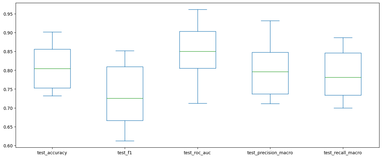
scores_df = pd.DataFrame(scores)scores_df.drop(columns=["fit_time", "score_time"]).plot(kind="box", figsize=(15, 6))
Let’s repeat this with a smaller number of folds.
model = XGBClassifier(random_state=42)

scores = cross_validate(
    model, X_train_val, y_train_val,
    scoring=['accuracy', 'f1', 'roc_auc', 'precision_macro', 'recall_macro'],
    n_jobs=-1,
    cv=5
    )

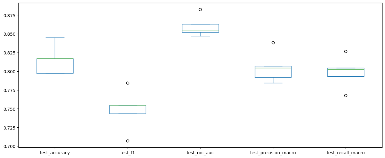
scores_df_5_fold = pd.DataFrame(scores)

scores_df_5_fold| fit_time | score_time | test_accuracy | test_f1 | test_roc_auc | test_precision_macro | test_recall_macro | |
|---|---|---|---|---|---|---|---|
| 0 | 0.146062 | 0.042184 | 0.797203 | 0.707071 | 0.852164 | 0.791950 | 0.767894 |
| 1 | 0.195811 | 0.051646 | 0.797203 | 0.743363 | 0.847170 | 0.784504 | 0.793383 |
| 2 | 0.244153 | 0.046421 | 0.845070 | 0.784314 | 0.882552 | 0.838271 | 0.826797 |
| 3 | 0.241028 | 0.049274 | 0.816901 | 0.754717 | 0.862943 | 0.804325 | 0.804325 |
| 4 | 0.261768 | 0.046865 | 0.816901 | 0.754717 | 0.854167 | 0.806838 | 0.802189 |
scores_df_5_fold.drop(columns=["fit_time", "score_time"]).plot(kind="box", figsize=(15, 6))
Let’s compare what we see.
scores_df_5_fold['folds'] = 5
scores_df['folds'] = 10

pd.concat([scores_df_5_fold, scores_df]).drop(columns=["fit_time", "score_time"]).plot(
    kind="box", figsize=(20, 6), by='folds'
    )
test_accuracy Axes(0.125,0.11;0.133621x0.77)
test_f1 Axes(0.285345,0.11;0.133621x0.77)
test_precision_macro Axes(0.44569,0.11;0.133621x0.77)
test_recall_macro Axes(0.606034,0.11;0.133621x0.77)
test_roc_auc Axes(0.766379,0.11;0.133621x0.77)
dtype: object
Roughly how many datapoints do we get in our validation portion of the dataset when we do this?
len(X_train_val) / 1071.2Roughly how many examples of each class would there be in our resulting datasets?
y_train_val.value_counts()/100.0 44.4
1.0 26.8
Name: Survived, dtype: float64Let’s compare this with 5-fold validation.
len(X_train_val) / 5142.4y_train_val.value_counts()/50.0 88.8
1.0 53.6
Name: Survived, dtype: float6431 Prediction
We can still create predictions when using cross validation.
y_pred_10 = cross_val_predict(
    model,
    X_train_val,
    y_train_val,
    cv=10,
)

y_pred_5 = cross_val_predict(
    model,
    X_train_val,
    y_train_val,
    cv=5,
)
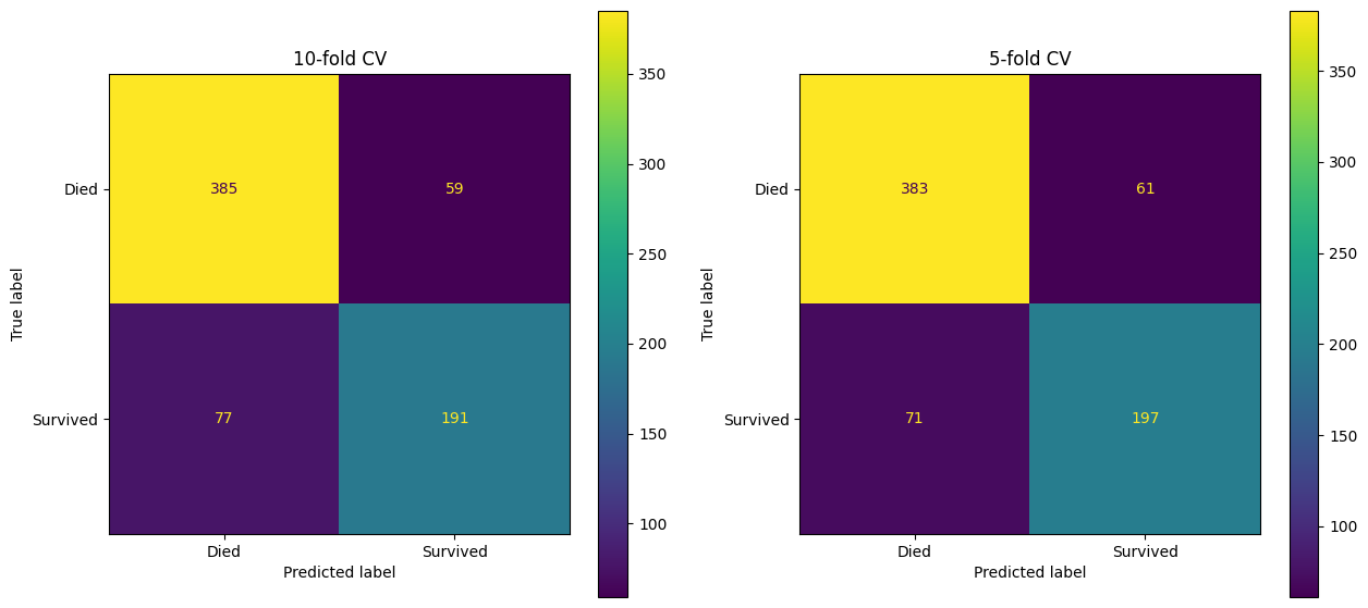
This allows us to create outputs like confusion matrices.
fig, (ax1, ax2) = plt.subplots(1, 2, figsize=(15, 7))

confusion_matrix_10 = ConfusionMatrixDisplay(
    confusion_matrix=confusion_matrix(
        y_true=y_train_val,
        y_pred=y_pred_10
        ),
        display_labels=["Died", "Survived"]

)

confusion_matrix_10.plot(ax=ax1)
ax1.set_title("10-fold CV")

confusion_matrix_5 = ConfusionMatrixDisplay(
    confusion_matrix=confusion_matrix(
        y_true=y_train_val,
        y_pred=y_pred_5
        ),
        display_labels=["Died", "Survived"]

)

confusion_matrix_5.plot(ax=ax2)
ax2.set_title("5-fold CV")
Text(0.5, 1.0, '5-fold CV')
Note the slight variation in performance here.
We can also generate performance reports.
pd.DataFrame(
    classification_report(y_train_val, y_pred_5, output_dict=True)
).round(3)| 0.0 | 1.0 | accuracy | macro avg | weighted avg | |
|---|---|---|---|---|---|
| precision | 0.844 | 0.764 | 0.815 | 0.804 | 0.813 |
| recall | 0.863 | 0.735 | 0.815 | 0.799 | 0.815 |
| f1-score | 0.853 | 0.749 | 0.815 | 0.801 | 0.814 |
| support | 444.000 | 268.000 | 0.815 | 712.000 | 712.000 |
32 Further Control
By setting up the KFold validation ourselves, we can have further control over the process.
Here, we are going to ensure the data is shuffled before use, and set a random seed so the process is replicable.
scores = cross_validate(
    model, X_train_val, y_train_val,
    scoring=['accuracy', 'f1', 'roc_auc', 'precision_macro', 'recall_macro'],
    n_jobs=-1,
    cv=StratifiedKFold(5, shuffle=True, random_state=42)
    )

scores_df_5_fold_shuffled_42 = pd.DataFrame(scores)

scores_df_5_fold_shuffled_42| fit_time | score_time | test_accuracy | test_f1 | test_roc_auc | test_precision_macro | test_recall_macro | |
|---|---|---|---|---|---|---|---|
| 0 | 1.316582 | 0.346691 | 0.783217 | 0.704762 | 0.831149 | 0.770354 | 0.763941 |
| 1 | 3.018813 | 0.269090 | 0.874126 | 0.823529 | 0.898772 | 0.874342 | 0.855181 |
| 2 | 1.302990 | 0.355363 | 0.823944 | 0.757282 | 0.853297 | 0.813913 | 0.806127 |
| 3 | 0.987926 | 0.197368 | 0.781690 | 0.704762 | 0.837821 | 0.766880 | 0.764787 |
| 4 | 0.566683 | 0.074188 | 0.830986 | 0.750000 | 0.828283 | 0.838571 | 0.799242 |
Let’s take a look at the impact of changing the random seed.
scores = cross_validate(
    model, X_train_val, y_train_val,
    scoring=['accuracy', 'f1', 'roc_auc', 'precision_macro', 'recall_macro'],
    n_jobs=-1,
    cv=StratifiedKFold(5, shuffle=True, random_state=101)
    )

scores_df_5_fold_shuffled_102 = pd.DataFrame(scores)

scores_df_5_fold_shuffled_102| fit_time | score_time | test_accuracy | test_f1 | test_roc_auc | test_precision_macro | test_recall_macro | |
|---|---|---|---|---|---|---|---|
| 0 | 0.221575 | 0.176622 | 0.776224 | 0.698113 | 0.815543 | 0.762363 | 0.758323 |
| 1 | 1.539527 | 0.315225 | 0.825175 | 0.752475 | 0.866729 | 0.820922 | 0.801290 |
| 2 | 1.212714 | 0.612245 | 0.760563 | 0.679245 | 0.810473 | 0.744117 | 0.744117 |
| 3 | 1.664313 | 0.329696 | 0.802817 | 0.740741 | 0.896544 | 0.788924 | 0.793089 |
| 4 | 1.536362 | 0.269400 | 0.838028 | 0.772277 | 0.872475 | 0.835946 | 0.815657 |
scores_df_5_fold_shuffled_42['seed'] = 42
scores_df_5_fold_shuffled_102['seed'] = 102

pd.concat([scores_df_5_fold_shuffled_42,scores_df_5_fold_shuffled_102]) \
    .drop(columns=["fit_time", "score_time"]) \
    .plot(kind="box", figsize=(20, 6), by='seed')
test_accuracy Axes(0.125,0.11;0.133621x0.77)
test_f1 Axes(0.285345,0.11;0.133621x0.77)
test_precision_macro Axes(0.44569,0.11;0.133621x0.77)
test_recall_macro Axes(0.606034,0.11;0.133621x0.77)
test_roc_auc Axes(0.766379,0.11;0.133621x0.77)
dtype: object
32.1 Leave-one-out
An extreme version of cross validation is leave-one-out validation, where only one datapoint at a time is used for evaluating the model, and the rest is used as training data.
This can be useful for very small datasets, but is more computationally intensive.
Leave-one-out tends to give us a more realistic idea of the performance in the real world, but can also lead to higher variance.
scores = cross_validate(
    model, X_train_val, y_train_val,
    scoring=['accuracy', 'f1', 'roc_auc', 'precision_macro', 'recall_macro'],
    n_jobs=-1,
    cv=KFold(len(X_train_val)-1)
    )

scores_df_leave_one_out = pd.DataFrame(scores)

scores_df_leave_one_out| fit_time | score_time | test_accuracy | test_f1 | test_roc_auc | test_precision_macro | test_recall_macro | |
|---|---|---|---|---|---|---|---|
| 0 | 1.777401 | 2.717442 | 1.0 | 0.0 | NaN | 1.0 | 1.0 |
| 1 | 3.770272 | 2.818617 | 0.0 | 0.0 | NaN | 0.0 | 0.0 |
| 2 | 3.055812 | 0.985970 | 1.0 | 0.0 | NaN | 1.0 | 1.0 |
| 3 | 4.052561 | 1.256033 | 1.0 | 0.0 | NaN | 1.0 | 1.0 |
| 4 | 3.003047 | 2.907689 | 0.0 | 0.0 | NaN | 0.0 | 0.0 |
| ... | ... | ... | ... | ... | ... | ... | ... |
| 706 | 0.062687 | 0.026082 | 1.0 | 1.0 | NaN | 1.0 | 1.0 |
| 707 | 0.117362 | 0.037119 | 1.0 | 0.0 | NaN | 1.0 | 1.0 |
| 708 | 0.160492 | 0.026065 | 1.0 | 0.0 | NaN | 1.0 | 1.0 |
| 709 | 0.156961 | 0.022564 | 1.0 | 1.0 | NaN | 1.0 | 1.0 |
| 710 | 0.063164 | 0.018045 | 1.0 | 0.0 | NaN | 1.0 | 1.0 |
711 rows × 7 columns
y_pred_leave_one_out = cross_val_predict(
    model,
    X_train_val,
    y_train_val,
    cv=KFold(len(X_train_val)-1),
)
fig, (ax1, ax2) = plt.subplots(1, 2, figsize=(15, 7))
confusion_matrix_10 = ConfusionMatrixDisplay(
confusion_matrix=confusion_matrix(
y_true=y_train_val,
y_pred=y_pred_leave_one_out
),
display_labels=["Died", "Survived"]
)
confusion_matrix_10.plot(ax=ax1)
ax1.set_title("Leave One Out")
confusion_matrix_5 = ConfusionMatrixDisplay(
confusion_matrix=confusion_matrix(
y_true=y_train_val,
y_pred=y_pred_5
),
display_labels=["Died", "Survived"]
)
confusion_matrix_5.plot(ax=ax2)
ax2.set_title("5-fold CV")Text(0.5, 1.0, '5-fold CV')
We can also generate other reports here.
pd.DataFrame(
    classification_report(y_train_val, y_pred_leave_one_out,
                          output_dict=True)
)| 0.0 | 1.0 | accuracy | macro avg | weighted avg | |
|---|---|---|---|---|---|
| precision | 0.839912 | 0.761719 | 0.811798 | 0.800816 | 0.810480 |
| recall | 0.862613 | 0.727612 | 0.811798 | 0.795112 | 0.811798 |
| f1-score | 0.851111 | 0.744275 | 0.811798 | 0.797693 | 0.810897 |
| support | 444.000000 | 268.000000 | 0.811798 | 712.000000 | 712.000000 |
