!pip install catboost
!pip install --upgrade scikit-learn
!git clone https://github.com/hsma-programme/h6_4g_explainable_ai.git
%cd /content/h6_4g_explainable_ai/solutions20 Exercise Solution: Explainable AI (LOS Dataset)
If using colab, run this cell first. Otherwise, skip this cell.
20.1 Core
We’re going to work with a dataset to try to predict patient length of stay.
import pandas as pd
import matplotlib.pyplot as plt
%matplotlib inline

# import the relevant models from Sklearn, XGBoost, CatBoost and LightGBM
from sklearn.linear_model import LinearRegression
from sklearn.tree import DecisionTreeRegressor
from sklearn.ensemble import RandomForestRegressor

from sklearn.preprocessing import StandardScaler
from sklearn.model_selection import train_test_split

from xgboost import XGBRegressor
from lightgbm import LGBMRegressor
from catboost import CatBoostRegressor
from sklearn.ensemble import HistGradientBoostingRegressor
# import any other libraries you need
import numpy as np
from sklearn.metrics import mean_absolute_error, mean_absolute_percentage_error, \
                            r2_score, root_mean_squared_error
# Additional imports for explainable AI
from sklearn.inspection import PartialDependenceDisplay, permutation_importance
# Import shap for shapley values
import shap
# JavaScript Important for the interactive charts later on
shap.initjs()Open the data dictionary in the los_dataset folder and take a look at what data is available.
Next, load in the dataframe containing the LOS data.
los_df = pd.read_csv("../datasets/los_dataset/LengthOfStay.csv", index_col="eid")View the dataframe.
los_df.head()| vdate | rcount | gender | dialysisrenalendstage | asthma | irondef | pneum | substancedependence | psychologicaldisordermajor | depress | ... | sodium | glucose | bloodureanitro | creatinine | bmi | pulse | respiration | secondarydiagnosisnonicd9 | facid | lengthofstay | |
|---|---|---|---|---|---|---|---|---|---|---|---|---|---|---|---|---|---|---|---|---|---|
| eid | |||||||||||||||||||||
| 1 | 8/29/2012 | 0 | F | 0 | 0 | 0 | 0 | 0 | 0 | 0 | ... | 140.361132 | 192.476918 | 12.0 | 1.390722 | 30.432418 | 96 | 6.5 | 4 | B | 3 |
| 2 | 5/26/2012 | 5+ | F | 0 | 0 | 0 | 0 | 0 | 0 | 0 | ... | 136.731692 | 94.078507 | 8.0 | 0.943164 | 28.460516 | 61 | 6.5 | 1 | A | 7 |
| 3 | 9/22/2012 | 1 | F | 0 | 0 | 0 | 0 | 0 | 0 | 0 | ... | 133.058514 | 130.530524 | 12.0 | 1.065750 | 28.843812 | 64 | 6.5 | 2 | B | 3 |
| 4 | 8/9/2012 | 0 | F | 0 | 0 | 0 | 0 | 0 | 0 | 0 | ... | 138.994023 | 163.377028 | 12.0 | 0.906862 | 27.959007 | 76 | 6.5 | 1 | A | 1 |
| 5 | 12/20/2012 | 0 | F | 0 | 0 | 0 | 1 | 0 | 1 | 0 | ... | 138.634836 | 94.886654 | 11.5 | 1.242854 | 30.258927 | 67 | 5.6 | 2 | E | 4 |
5 rows × 26 columns
Consider what columns to remove.
HINT: Is there a column in the dataset that doesn’t really make much sense to predict from? If you’re not sure, use the full dataset for now and come back to this later.
NOTE: For now, we’re going to assume that all of the included measures will be available to us at the point we need to make a prediction - they’re not things that will be calculated later in the patient’s stay.
los_df = los_df.drop(columns="vdate")
los_df.head(1)| rcount | gender | dialysisrenalendstage | asthma | irondef | pneum | substancedependence | psychologicaldisordermajor | depress | psychother | ... | sodium | glucose | bloodureanitro | creatinine | bmi | pulse | respiration | secondarydiagnosisnonicd9 | facid | lengthofstay | |
|---|---|---|---|---|---|---|---|---|---|---|---|---|---|---|---|---|---|---|---|---|---|
| eid | |||||||||||||||||||||
| 1 | 0 | F | 0 | 0 | 0 | 0 | 0 | 0 | 0 | 0 | ... | 140.361132 | 192.476918 | 12.0 | 1.390722 | 30.432418 | 96 | 6.5 | 4 | B | 3 |
1 rows × 25 columns
Convert categories with only two options into a boolean value (e.g. for a gender column in which gender has only been provided as M or F, you could encode M as 0 and F as 1).
los_df.gender.unique()array(['F', 'M'], dtype=object)los_df['gender'].replace('M', 0, inplace=True)
los_df['gender'].replace('F', 1, inplace=True)
los_df.gender.unique()array([1, 0], dtype=int64)Convert columns with multiple options per category into multiple columns using one-hot encoding.
los_df.facid.unique()

# Bonus - astype('int') will convert the true/false values to 0/1
# not necessary - it will work regardless
one_hot = pd.get_dummies(los_df['facid']).astype('int')
los_df = los_df.drop('facid', axis=1)
los_df = los_df.join(one_hot)los_df.head()| rcount | gender | dialysisrenalendstage | asthma | irondef | pneum | substancedependence | psychologicaldisordermajor | depress | psychother | ... | bmi | pulse | respiration | secondarydiagnosisnonicd9 | lengthofstay | A | B | C | D | E | |
|---|---|---|---|---|---|---|---|---|---|---|---|---|---|---|---|---|---|---|---|---|---|
| eid | |||||||||||||||||||||
| 1 | 0 | 1 | 0 | 0 | 0 | 0 | 0 | 0 | 0 | 0 | ... | 30.432418 | 96 | 6.5 | 4 | 3 | 0 | 1 | 0 | 0 | 0 |
| 2 | 5+ | 1 | 0 | 0 | 0 | 0 | 0 | 0 | 0 | 0 | ... | 28.460516 | 61 | 6.5 | 1 | 7 | 1 | 0 | 0 | 0 | 0 |
| 3 | 1 | 1 | 0 | 0 | 0 | 0 | 0 | 0 | 0 | 0 | ... | 28.843812 | 64 | 6.5 | 2 | 3 | 0 | 1 | 0 | 0 | 0 |
| 4 | 0 | 1 | 0 | 0 | 0 | 0 | 0 | 0 | 0 | 0 | ... | 27.959007 | 76 | 6.5 | 1 | 1 | 1 | 0 | 0 | 0 | 0 |
| 5 | 0 | 1 | 0 | 0 | 0 | 1 | 0 | 1 | 0 | 0 | ... | 30.258927 | 67 | 5.6 | 2 | 4 | 0 | 0 | 0 | 0 | 1 |
5 rows × 29 columns
los_df.rcount.value_counts()

# Bonus - astype('int') will convert the true/false values to 0/1
# not necessary - it will work regardless
one_hot = pd.get_dummies(los_df['rcount'], prefix="rcount").astype('int')
los_df = los_df.drop('rcount', axis=1)
los_df = los_df.join(one_hot)
los_df.head()| gender | dialysisrenalendstage | asthma | irondef | pneum | substancedependence | psychologicaldisordermajor | depress | psychother | fibrosisandother | ... | B | C | D | E | rcount_0 | rcount_1 | rcount_2 | rcount_3 | rcount_4 | rcount_5+ | |
|---|---|---|---|---|---|---|---|---|---|---|---|---|---|---|---|---|---|---|---|---|---|
| eid | |||||||||||||||||||||
| 1 | 1 | 0 | 0 | 0 | 0 | 0 | 0 | 0 | 0 | 0 | ... | 1 | 0 | 0 | 0 | 1 | 0 | 0 | 0 | 0 | 0 |
| 2 | 1 | 0 | 0 | 0 | 0 | 0 | 0 | 0 | 0 | 0 | ... | 0 | 0 | 0 | 0 | 0 | 0 | 0 | 0 | 0 | 1 |
| 3 | 1 | 0 | 0 | 0 | 0 | 0 | 0 | 0 | 0 | 0 | ... | 1 | 0 | 0 | 0 | 0 | 1 | 0 | 0 | 0 | 0 |
| 4 | 1 | 0 | 0 | 0 | 0 | 0 | 0 | 0 | 0 | 0 | ... | 0 | 0 | 0 | 0 | 1 | 0 | 0 | 0 | 0 | 0 |
| 5 | 1 | 0 | 0 | 0 | 1 | 0 | 1 | 0 | 0 | 0 | ... | 0 | 0 | 0 | 1 | 1 | 0 | 0 | 0 | 0 | 0 |
5 rows × 34 columns
Train a decision tree model to predict length of stay based on the variables in this dataset.
X = los_df.drop(columns='lengthofstay')
y = los_df['lengthofstay']

X_train, X_test, y_train, y_test = train_test_split(
    X, y,
    test_size = 0.25,
    random_state=42
    )

regr_dt = DecisionTreeRegressor(random_state=42)

# Train the model using the training sets
regr_dt.fit(X_train, y_train)

# Make predictions using the testing set
y_pred_train = regr_dt.predict(X_train)
y_pred_test = regr_dt.predict(X_test)y_pred_testarray([3., 1., 3., ..., 8., 2., 5.])Assess the performance of this model.
print("TRAINING DATA")
print(f"Mean absolute error: {mean_absolute_error(y_train, y_pred_train):.2f}")
print(f"Mean absolute percentage error: {mean_absolute_percentage_error(y_train, y_pred_train):.2%}" )
print("Root Mean squared error: %.2f" % root_mean_squared_error(y_train, y_pred_train))
# The coefficient of determination: 1 is perfect prediction
print("Coefficient of determination: %.2f" % r2_score(y_train, y_pred_train))
TRAINING DATA
Mean absolute error: 0.00
Mean absolute percentage error: 0.00%
Root Mean squared error: 0.00
Coefficient of determination: 1.00print("TESTING DATA")
print(f"Mean absolute error: {mean_absolute_error(y_test, y_pred_test):.2f}")
print(f"Mean absolute percentage error: {mean_absolute_percentage_error(y_test, y_pred_test):.2%}" )
print("Root Mean squared error: %.2f" % root_mean_squared_error(y_test, y_pred_test))
# The coefficient of determination: 1 is perfect prediction
print("Coefficient of determination: %.2f" % r2_score(y_test, y_pred_test))TESTING DATA
Mean absolute error: 0.50
Mean absolute percentage error: 12.94%
Root Mean squared error: 0.93
Coefficient of determination: 0.84def plot_residuals(actual, predicted):
residuals = actual - predicted
plt.figure(figsize=(10, 5))
plt.hist(residuals, bins=20)
plt.axvline(x = 0, color = 'r')
plt.xlabel('Residual')
plt.ylabel('Frequency')
plt.title('Distribution of Residuals')
plt.show()
plot_residuals(y_test, y_pred_test)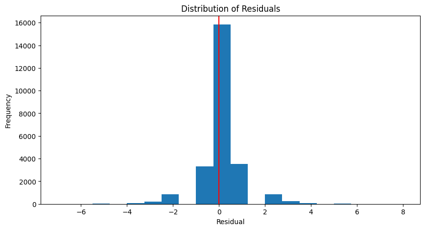
def plot_actual_vs_predicted(actual, predicted):
    fig, ax = plt.subplots(figsize=(6, 6))

    ax.scatter(actual, predicted, color="black", alpha=0.05)
    ax.axline((1, 1), slope=1)
    plt.xlabel('True Values')
    plt.ylabel('Predicted Values')
    plt.title('True vs Predicted Values')
    plt.show()

plot_actual_vs_predicted(y_test, y_pred_test)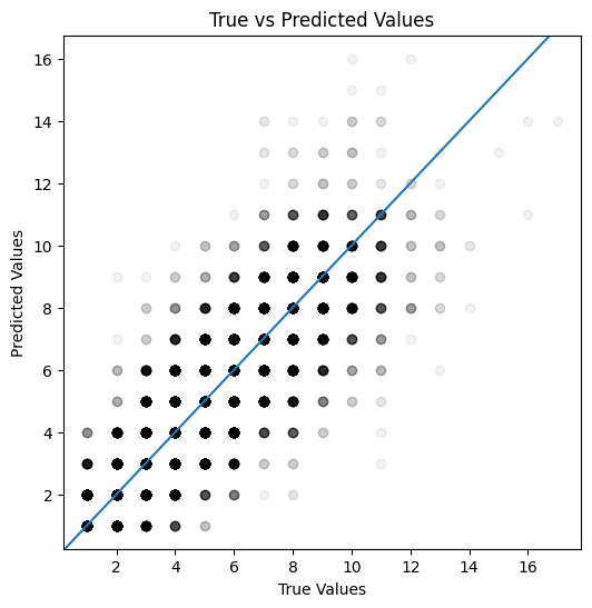
Train a boosting model to predict length of stay based on the variables in this dataset.
X = los_df.drop(columns='lengthofstay')
y = los_df['lengthofstay']

X_train, X_test, y_train, y_test = train_test_split(
    X, y,
    test_size = 0.25,
    random_state=42
    )

regr_xgb = XGBRegressor(random_state=42)

# Train the model using the training sets
regr_xgb.fit(X_train, y_train)

# Make predictions using the testing set
y_pred_train = regr_xgb.predict(X_train)
y_pred_test = regr_xgb.predict(X_test)y_pred_testarray([3.6313417, 0.8304186, 2.4800673, ..., 5.5354204, 1.5881324,
5.249632 ], dtype=float32)Assess the performance of this model and compare it with your decision tree model.
print("TRAINING DATA")
print(f"Mean absolute error: {mean_absolute_error(y_train, y_pred_train):.2f}")
print(f"Mean absolute percentage error: {mean_absolute_percentage_error(y_train, y_pred_train):.2%}" )
print("Root Mean squared error: %.2f" % root_mean_squared_error(y_train, y_pred_train))
# The coefficient of determination: 1 is perfect prediction
print("Coefficient of determination: %.2f" % r2_score(y_train, y_pred_train))
TRAINING DATA
Mean absolute error: 0.29
Mean absolute percentage error: 10.66%
Root Mean squared error: 0.37
Coefficient of determination: 0.98print("TESTING DATA")
print(f"Mean absolute error: {mean_absolute_error(y_test, y_pred_test):.2f}")
print(f"Mean absolute percentage error: {mean_absolute_percentage_error(y_test, y_pred_test):.2%}" )
print("Root Mean squared error: %.2f" % root_mean_squared_error(y_test, y_pred_test))
# The coefficient of determination: 1 is perfect prediction
print("Coefficient of determination: %.2f" % r2_score(y_test, y_pred_test))TESTING DATA
Mean absolute error: 0.33
Mean absolute percentage error: 11.60%
Root Mean squared error: 0.44
Coefficient of determination: 0.96plot_residuals(y_test, y_pred_test)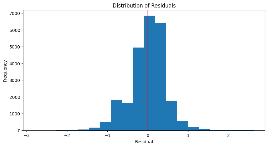
plot_actual_vs_predicted(y_test, y_pred_test)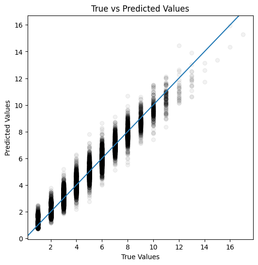
20.2 Exercise 4G: Explainable AI
20.2.1 Explore feature importance
20.2.1.1 Importance with MDI
features = list(X_train)

feature_importances_dt = regr_dt.feature_importances_
importances_dt = pd.DataFrame(index=features)
importances_dt['importance_dt'] = feature_importances_dt
importances_dt['rank_dt'] = importances_dt['importance_dt'].rank(ascending=False).values
importances_dt.sort_values('rank_dt').head()| importance_dt | rank_dt | |
|---|---|---|
| rcount_0 | 0.358057 | 1.0 |
| rcount_1 | 0.140998 | 2.0 |
| E | 0.114736 | 3.0 |
| hematocrit | 0.044496 | 4.0 |
| rcount_2 | 0.040130 | 5.0 |
feature_importances_xgb = regr_xgb.feature_importances_
importances_xgb = pd.DataFrame(index=features)
importances_xgb['importance_xgb'] = feature_importances_xgb
importances_xgb['rank_xgb'] = importances_xgb['importance_xgb'].rank(ascending=False).values
importances_xgb.sort_values('rank_xgb').head()| importance_xgb | rank_xgb | |
|---|---|---|
| rcount_0 | 0.298638 | 1.0 |
| rcount_1 | 0.223313 | 2.0 |
| E | 0.104948 | 3.0 |
| rcount_2 | 0.095113 | 4.0 |
| rcount_3 | 0.044833 | 5.0 |
20.2.2 Repeat using PFI
feature_names = X.columns.tolist()

result_dt_pfi = permutation_importance(
    regr_dt, X_test, y_test, n_repeats=10, random_state=42, n_jobs=2
)

importances_pfi_dt = pd.Series(result_dt_pfi.importances_mean, index=feature_names)

fig, ax = plt.subplots(figsize=(15,10))
importances_pfi_dt.plot.bar(yerr=result_dt_pfi.importances_std, ax=ax)
ax.set_title("Feature importances using permutation on full model")
ax.set_ylabel("Mean accuracy decrease")
fig.tight_layout()
plt.show()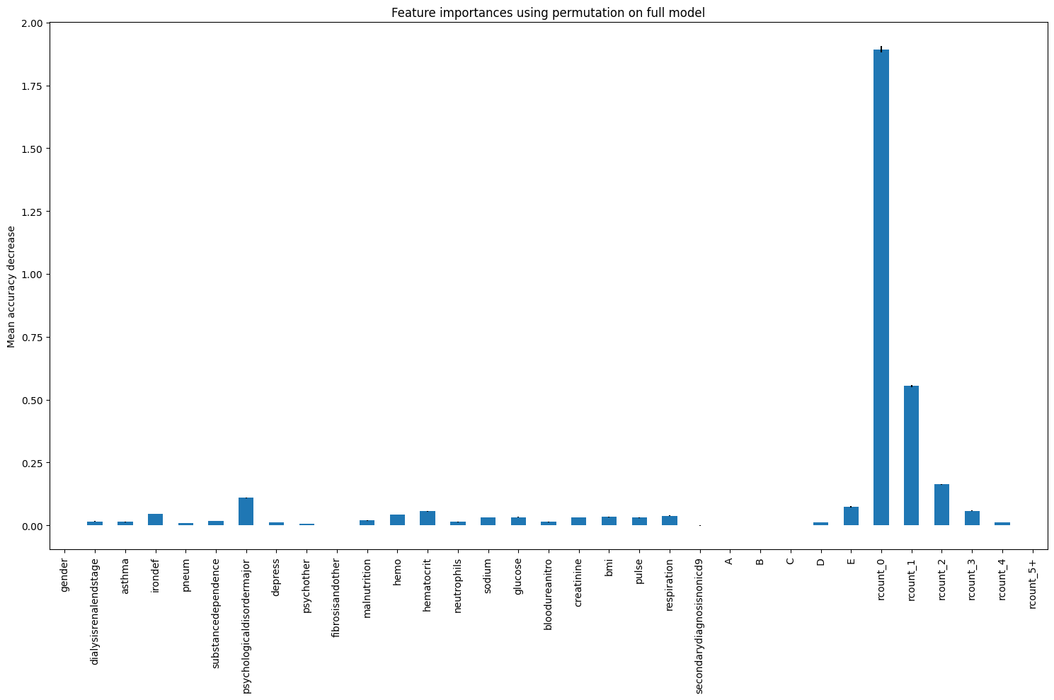
feature_names = X.columns.tolist()

result_xgb_pfi = permutation_importance(
    regr_xgb, X_test, y_test, n_repeats=10, random_state=42, n_jobs=2
)

importances_pfi_xgb = pd.Series(result_xgb_pfi.importances_mean, index=feature_names)

fig, ax = plt.subplots(figsize=(15,10))
importances_pfi_xgb.plot.bar(yerr=result_xgb_pfi.importances_std, ax=ax)
ax.set_title("Feature importances using permutation on full model")
ax.set_ylabel("Mean accuracy decrease")
fig.tight_layout()
plt.show()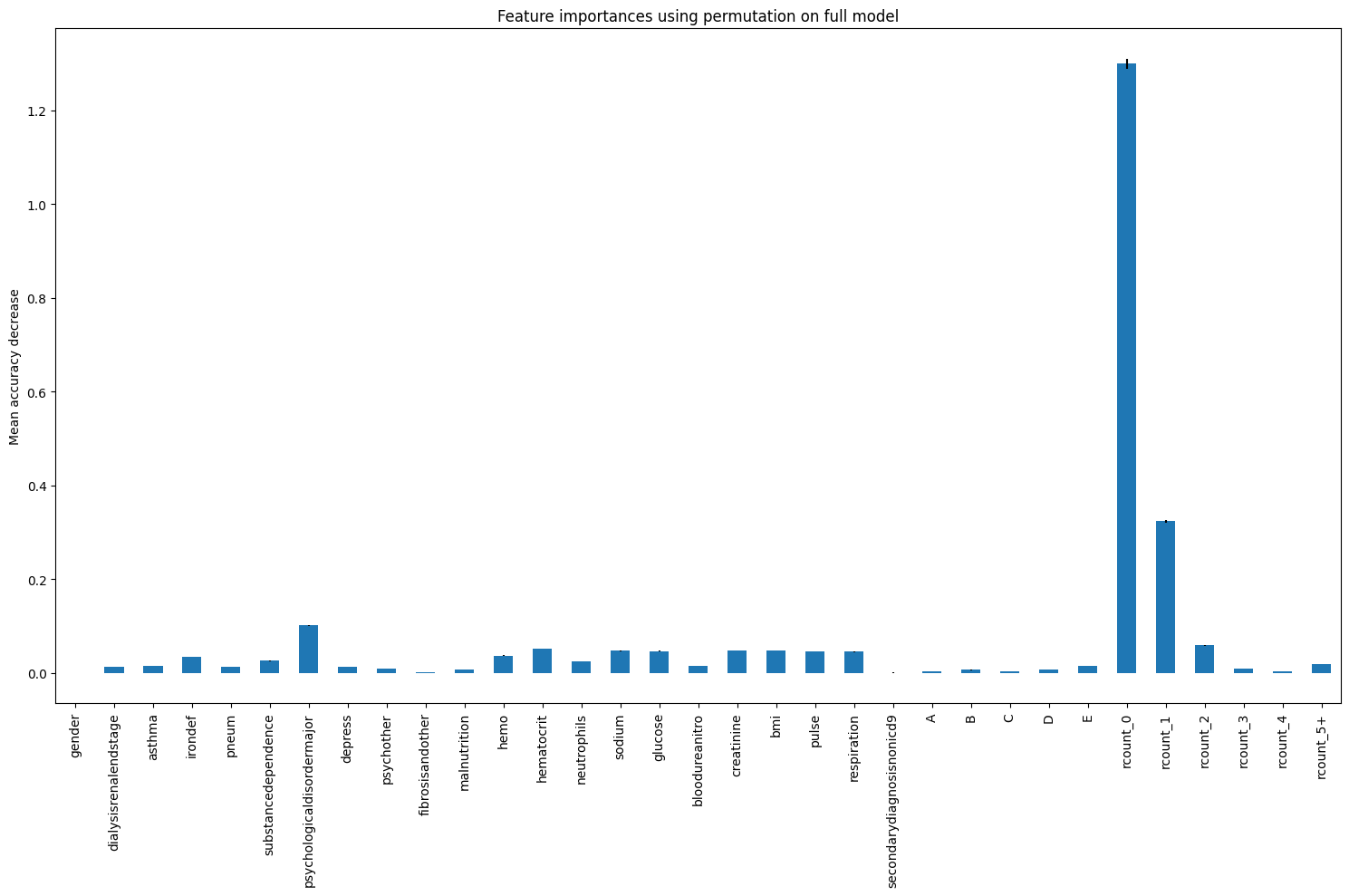
20.3 SHAP
All code below has just been applied to the xg boost version of the model.
When do we pass in different bits of data?
The foreground data is the input to explainer.shap_values and the background data is the data parameter of shap.TreeExplainer’s init.
If you don’t input foreground data you won’t get SHAP values, so it wouldn’t make much sense to not input foreground data.
If you don’t input the background data, it will actually use a different version of TreeExplainer (path dependent) that implicitly uses the training data as the background data set.
- Hugh Chen, https://github.com/shap/shap/issues/1366
# explain the model's predictions using SHAP
explainer = shap.Explainer(regr_xgb, X_train)

shap_values = explainer(X_test)

shap_values
99%|===================| 24754/25000 [00:49<00:00] .values =
array([[ 0.00764417, 0. , -0.03838515, ..., 0.02178417,
-0.01230581, -0.05431815],
[ 0.00406493, 0. , -0.08355626, ..., 0.02667989,
-0.01247949, -0.05238643],
[-0.00260847, 0. , -0.07398675, ..., 0.02891657,
-0.01341456, -0.05173721],
...,
[-0.00061298, 0. , -0.03833514, ..., 0.02290138,
-0.0153973 , -0.05772406],
[-0.00180168, 0. , -0.06790128, ..., 0.02414472,
-0.01215895, -0.05733014],
[ 0.00211131, 0. , -0.04626162, ..., 0.02808055,
-0.00878728, -0.045735 ]])
.base_values =
array([3.79460651, 3.79460651, 3.79460651, ..., 3.79460651, 3.79460651,
3.79460651])
.data =
array([[0., 0., 0., ..., 0., 0., 0.],
[0., 0., 0., ..., 0., 0., 0.],
[1., 0., 0., ..., 0., 0., 0.],
...,
[0., 0., 0., ..., 0., 0., 0.],
[1., 0., 0., ..., 0., 0., 0.],
[0., 0., 0., ..., 0., 0., 0.]])20.3.0.1 Returning just the values
It can be useful to have access to just the shap values in an object as they are required as the input to some steps.
Note that we have used ‘shap_values’ as the variable to store the output of explainer(). So we will need to give it another name!
shap_values_numeric = shap_values.values
shap_values_numeric
array([[ 0.00764417, 0. , -0.03838515, ..., 0.02178417,
-0.01230581, -0.05431815],
[ 0.00406493, 0. , -0.08355626, ..., 0.02667989,
-0.01247949, -0.05238643],
[-0.00260847, 0. , -0.07398675, ..., 0.02891657,
-0.01341456, -0.05173721],
...,
[-0.00061298, 0. , -0.03833514, ..., 0.02290138,
-0.0153973 , -0.05772406],
[-0.00180168, 0. , -0.06790128, ..., 0.02414472,
-0.01215895, -0.05733014],
[ 0.00211131, 0. , -0.04626162, ..., 0.02808055,
-0.00878728, -0.045735 ]])20.3.0.2 Feature Table
# get feature importance for comparison using MDI method
features = list(X_train)
feature_importances = regr_xgb.feature_importances_
importances = pd.DataFrame(index=features)
importances['importance'] = feature_importances
importances['rank'] = importances['importance'].rank(ascending=False).values
importances.sort_values('rank').head()

# Get shapley importances
# Calculate mean Shapley value for each feature in trainign set
importances['mean_shapley_values'] = np.mean(
    shap_values_numeric, axis=0
    )

# Calculate mean absolute Shapley value for each feature in trainign set
# This will give us the average importance of each feature
importances['mean_abs_shapley_values'] = np.mean(
    np.abs(shap_values_numeric), axis=0
    )

importances| importance | rank | mean_shapley_values | mean_abs_shapley_values | |
|---|---|---|---|---|
| gender | 0.000152 | 33.0 | 0.000497 | 0.003516 |
| dialysisrenalendstage | 0.004975 | 23.0 | 0.022847 | 0.022847 |
| asthma | 0.004017 | 25.0 | -0.029080 | 0.084459 |
| irondef | 0.016412 | 9.0 | -0.016085 | 0.134217 |
| pneum | 0.006473 | 16.0 | 0.027612 | 0.027612 |
| substancedependence | 0.005187 | 19.0 | -0.031714 | 0.132673 |
| psychologicaldisordermajor | 0.014801 | 10.0 | 0.014358 | 0.361950 |
| depress | 0.002699 | 28.0 | -0.025356 | 0.082002 |
| psychother | 0.001460 | 29.0 | 0.009927 | 0.046745 |
| fibrosisandother | 0.002701 | 27.0 | -0.001231 | 0.006100 |
| malnutrition | 0.005148 | 20.0 | 0.012160 | 0.029192 |
| hemo | 0.020425 | 8.0 | -0.007621 | 0.122109 |
| hematocrit | 0.008906 | 12.0 | 0.027616 | 0.265825 |
| neutrophils | 0.003719 | 26.0 | 0.006639 | 0.125201 |
| sodium | 0.005029 | 21.0 | 0.018857 | 0.254019 |
| glucose | 0.005008 | 22.0 | 0.052205 | 0.235265 |
| bloodureanitro | 0.007172 | 15.0 | 0.038006 | 0.056848 |
| creatinine | 0.004722 | 24.0 | -0.030582 | 0.275831 |
| bmi | 0.005255 | 18.0 | 0.033641 | 0.254814 |
| pulse | 0.006221 | 17.0 | -0.011668 | 0.261527 |
| respiration | 0.008615 | 13.0 | 0.003487 | 0.236613 |
| secondarydiagnosisnonicd9 | 0.000228 | 32.0 | 0.000217 | 0.002621 |
| A | 0.001182 | 30.0 | -0.005640 | 0.031220 |
| B | 0.000977 | 31.0 | -0.003409 | 0.042982 |
| C | 0.008053 | 14.0 | -0.006742 | 0.026159 |
| D | 0.028479 | 7.0 | -0.000704 | 0.021886 |
| E | 0.104948 | 3.0 | -0.001272 | 0.065105 |
| rcount_0 | 0.298638 | 1.0 | 0.142340 | 1.741959 |
| rcount_1 | 0.223313 | 2.0 | -0.021455 | 0.514860 |
| rcount_2 | 0.095113 | 4.0 | -0.020626 | 0.171157 |
| rcount_3 | 0.044833 | 5.0 | -0.003072 | 0.054635 |
| rcount_4 | 0.014782 | 11.0 | 0.007687 | 0.031047 |
| rcount_5+ | 0.040360 | 6.0 | -0.015835 | 0.098719 |
importance_top_10 = \
    importances.sort_values(
        by='importance', ascending=False
        ).head(10).index

shapley_top_10 = \
    importances.sort_values(
        by='mean_abs_shapley_values',
        ascending=False).head(10).index

# Add to DataFrame
top_10_features = pd.DataFrame()
top_10_features['importances'] = importance_top_10.values
top_10_features['Shapley'] = shapley_top_10.values

# Display
top_10_features| importances | Shapley | |
|---|---|---|
| 0 | rcount_0 | rcount_0 |
| 1 | rcount_1 | rcount_1 |
| 2 | E | psychologicaldisordermajor |
| 3 | rcount_2 | creatinine |
| 4 | rcount_3 | hematocrit |
| 5 | rcount_5+ | pulse |
| 6 | D | bmi |
| 7 | hemo | sodium |
| 8 | irondef | respiration |
| 9 | psychologicaldisordermajor | glucose |
20.3.1 Global: Beeswarm
# summarize the effects of all the features
shap.plots.beeswarm(shap_values, max_display=25)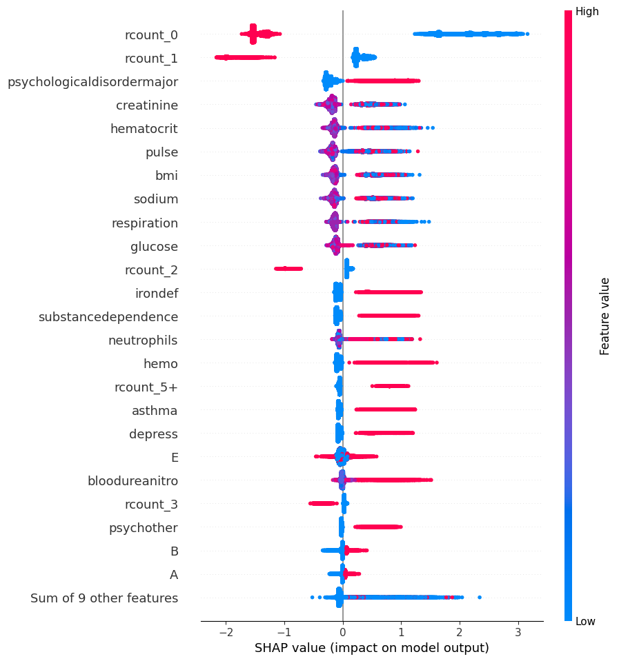
20.3.2 Global: Bar
shap.plots.bar(shap_values, max_display=20)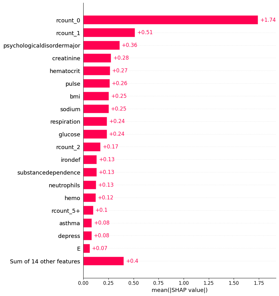
20.3.2.1 Bar: by another factor
Here we are creating a bar chart by another cohort.
We can see there is almost no gender difference in this dataset.
sex = ["Women" if shap_values[i, "gender"].data == 1 else "Men" for i in range(shap_values.shape[0])]
shap.plots.bar(shap_values.cohorts(sex).abs.mean(0))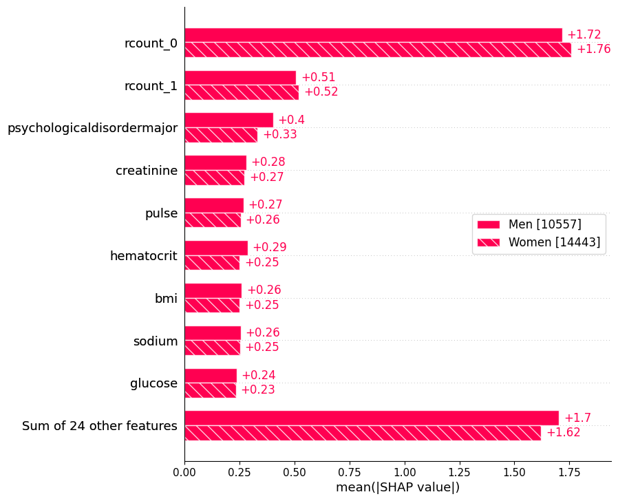
readmission_status = ["Not Readmitted" if shap_values[i, "rcount_0"].data == 1 else "Readmitted" for i in range(shap_values.shape[0])]
shap.plots.bar(shap_values.cohorts(readmission_status).abs.mean(0), max_display=25)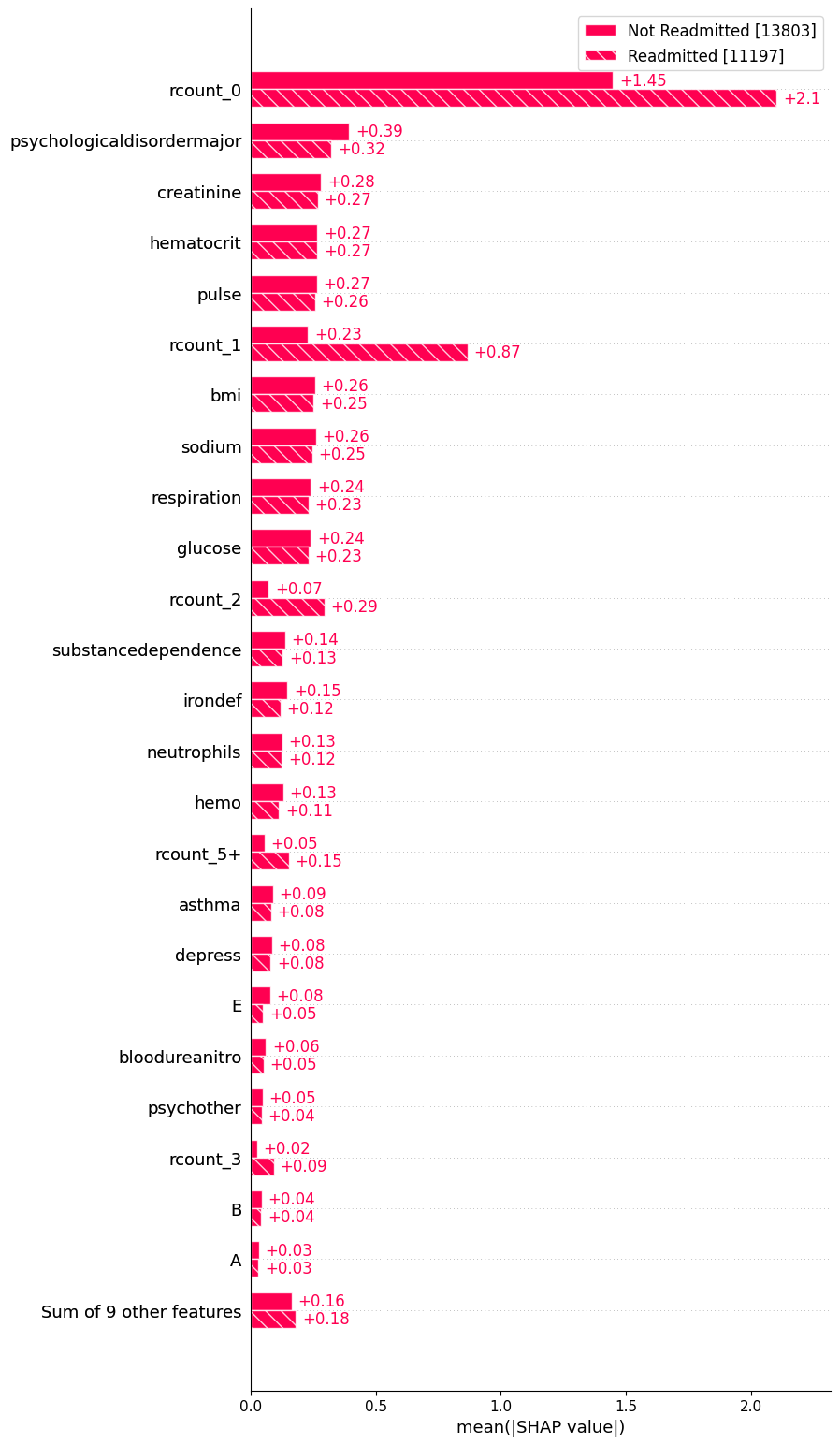
20.3.3 Local: Waterfall Plots
# visualize the first prediction's explanation
shap.plots.waterfall(shap_values[0])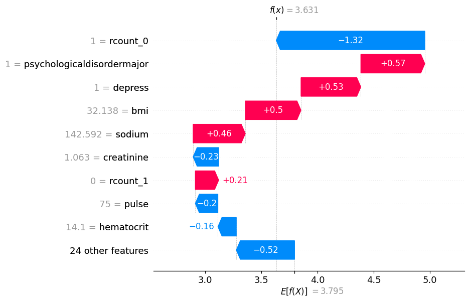
# visualize another prediction's explanation
shap.plots.waterfall(shap_values[7], max_display=15)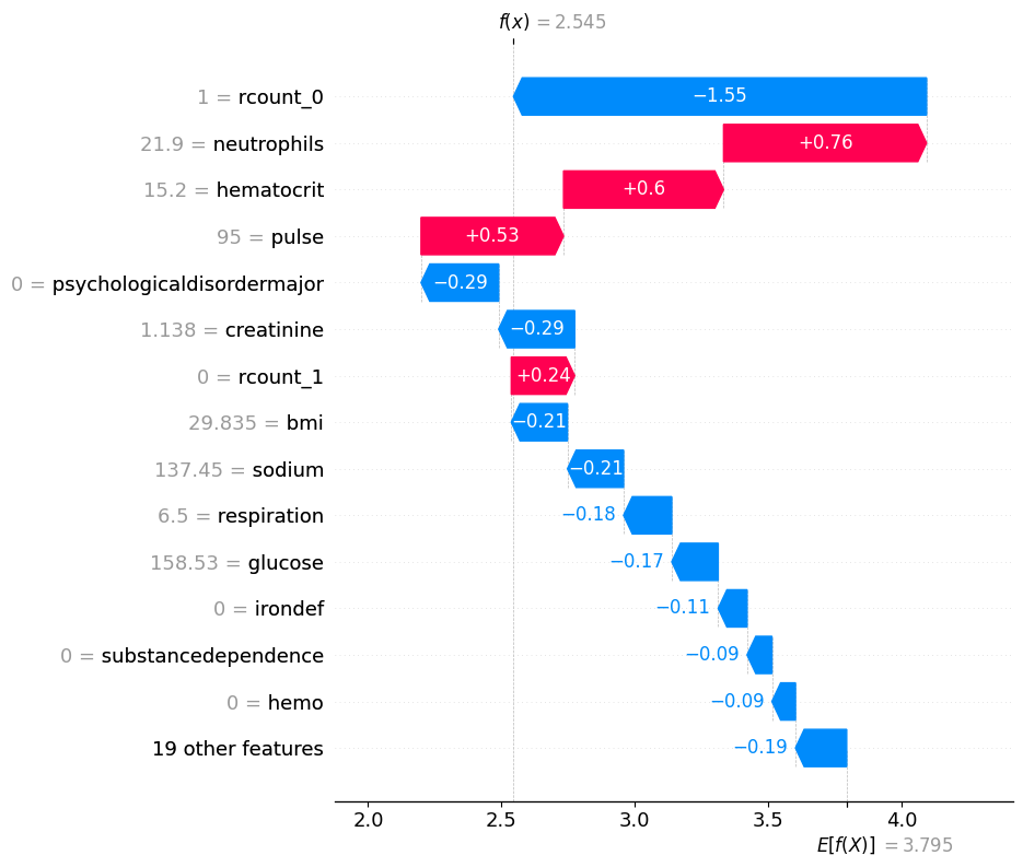
20.3.3.1 Visualise an example with a high LoS
highest_los = los_df.sort_values('lengthofstay', ascending=False).head(1)

high_los_index = highest_los.index
highest_los.lengthofstay
eid
7493 17
Name: lengthofstay, dtype: int64shap.plots.waterfall(shap_values[7493], max_display=15)
20.3.3.2 Visualise an example with a low LoS
shap.plots.waterfall(shap_values[y_test.reset_index(drop=True).sort_values().head(1).index[0]], max_display=20)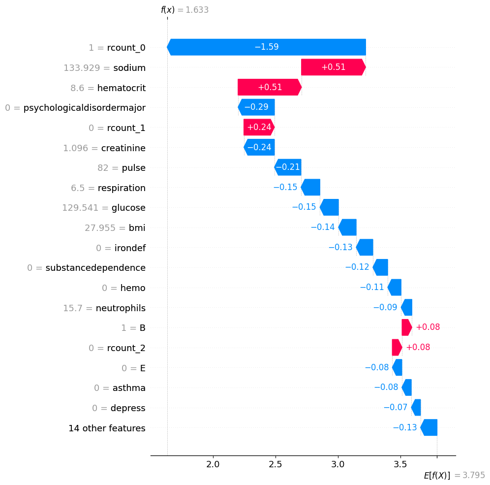
20.3.3.3 Visualise an example with a high LoS
shap.plots.waterfall(shap_values[y_test.reset_index(drop=True).sort_values().tail(1).index[0]], max_display=20)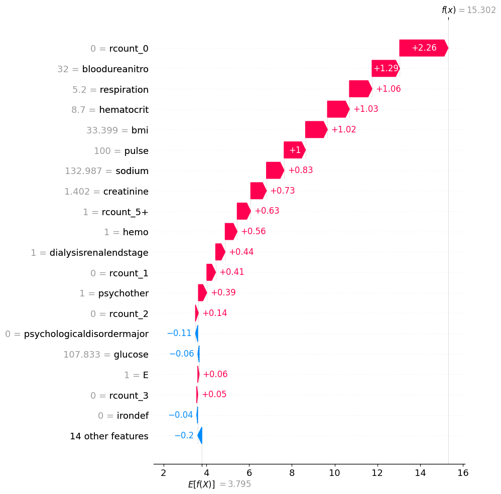
20.3.4 Local: Force Plots
# visualize the first prediction's explanation with a force plot
shap.plots.force(shap_values[0])Have you run `initjs()` in this notebook? If this notebook was from another user you must also trust this notebook (File -> Trust notebook). If you are viewing this notebook on github the Javascript has been stripped for security. If you are using JupyterLab this error is because a JupyterLab extension has not yet been written.
shap.plots.force(shap_values[y_test.reset_index(drop=True).sort_values().head(1).index[0]])Have you run `initjs()` in this notebook? If this notebook was from another user you must also trust this notebook (File -> Trust notebook). If you are viewing this notebook on github the Javascript has been stripped for security. If you are using JupyterLab this error is because a JupyterLab extension has not yet been written.
shap.plots.force(shap_values[y_test.reset_index(drop=True).sort_values().tail(1).index[0]])Have you run `initjs()` in this notebook? If this notebook was from another user you must also trust this notebook (File -> Trust notebook). If you are viewing this notebook on github the Javascript has been stripped for security. If you are using JupyterLab this error is because a JupyterLab extension has not yet been written.
0        3.631342
1        0.830419
2        2.480067
3        1.077456
4        5.112955
           ...
24995    7.090035
24996    1.122499
24997    5.535420
24998    1.588132
24999    5.249632
Length: 25000, dtype: float32
20.3.4.1 Visualise the lowest predicted LoS
shap.plots.force(shap_values[pd.Series(y_pred_test).sort_values().head(1).index[0]])Have you run `initjs()` in this notebook? If this notebook was from another user you must also trust this notebook (File -> Trust notebook). If you are viewing this notebook on github the Javascript has been stripped for security. If you are using JupyterLab this error is because a JupyterLab extension has not yet been written.
20.3.4.2 Visualise the highest predicted LoS
shap.plots.force(shap_values[pd.Series(y_pred_test).sort_values().tail(1).index[0]])Have you run `initjs()` in this notebook? If this notebook was from another user you must also trust this notebook (File -> Trust notebook). If you are viewing this notebook on github the Javascript has been stripped for security. If you are using JupyterLab this error is because a JupyterLab extension has not yet been written.
20.3.5 Global: Force Plots
# visualize all the predictions
# this struggles with a large number of values so we'll sample a small set
shap.plots.force(shap.utils.sample(shap_values, 1000))Have you run `initjs()` in this notebook? If this notebook was from another user you must also trust this notebook (File -> Trust notebook). If you are viewing this notebook on github the Javascript has been stripped for security. If you are using JupyterLab this error is because a JupyterLab extension has not yet been written.
20.3.6 Dependence Plots
20.3.6.1 Simple scatter of a single feature
# create a dependence scatter plot to show the effect of a single feature across the whole dataset
shap.plots.scatter(shap_values[:, 'respiration'])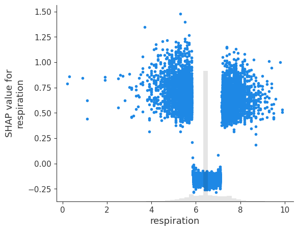
20.3.7 Scatter of multiple features
Passing in shap_values to the colour will colour the value by the most strongly interacting other value.
# create a dependence scatter plot to show the effect of a single feature across the whole dataset
shap.plots.scatter(shap_values[:, "gender"], color=shap_values)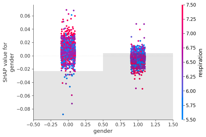
# create a dependence scatter plot to show the effect of a single feature across the whole dataset
shap.plots.scatter(shap_values[:, "respiration"], color=shap_values)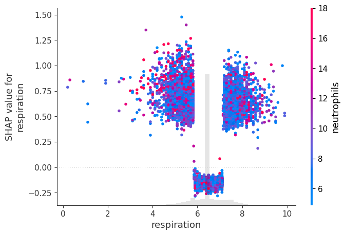
Alternatively we can choose to colour by a specific column.
X.columnsIndex(['gender', 'dialysisrenalendstage', 'asthma', 'irondef', 'pneum',
'substancedependence', 'psychologicaldisordermajor', 'depress',
'psychother', 'fibrosisandother', 'malnutrition', 'hemo', 'hematocrit',
'neutrophils', 'sodium', 'glucose', 'bloodureanitro', 'creatinine',
'bmi', 'pulse', 'respiration', 'secondarydiagnosisnonicd9', 'A', 'B',
'C', 'D', 'E', 'rcount_0', 'rcount_1', 'rcount_2', 'rcount_3',
'rcount_4', 'rcount_5+'],
dtype='object')# create a dependence scatter plot to show the effect of a single feature across the whole dataset
shap.plots.scatter(shap_values[:, "sodium"], color=shap_values[:,"glucose"])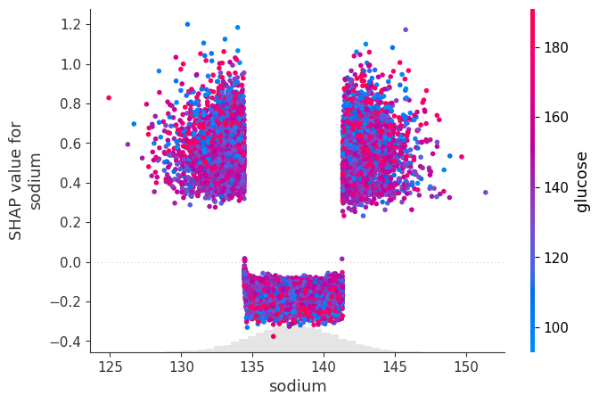
# create a dependence scatter plot to show the effect of a single feature across the whole dataset
shap.plots.scatter(shap_values[:, "rcount_1"], color=shap_values[:,"gender"])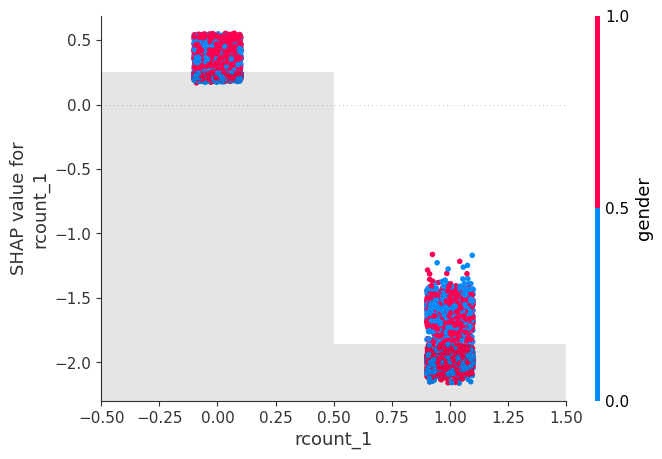
20.3.8 BONUS: SHAP interactions
Full details of SHAP interactions can be found here: https://michaelallen1966.github.io/titanic/90_shap_interactions_on_titanic.html
First we need to get the interaction values from the explainer object. Like before, we pass in our foreground data. The interactions take a long time to calculate, even using xgboost, so I’ve just asked for 1000.
shap_interaction = explainer.shap_interaction_values(shap.utils.sample(X, 1000))shap_interaction.shape(1000, 33, 33)20.3.8.1 Table
mean_abs_interactions = pd.DataFrame(
    np.abs(shap_interaction).mean(axis=(0)),
    index=X.columns, columns=X.columns)

mean_abs_interactions.round(2)| gender | dialysisrenalendstage | asthma | irondef | pneum | substancedependence | psychologicaldisordermajor | depress | psychother | fibrosisandother | ... | B | C | D | E | rcount_0 | rcount_1 | rcount_2 | rcount_3 | rcount_4 | rcount_5+ | |
|---|---|---|---|---|---|---|---|---|---|---|---|---|---|---|---|---|---|---|---|---|---|
| gender | 0.0 | 0.0 | 0.0 | 0.0 | 0.0 | 0.0 | 0.0 | 0.0 | 0.0 | 0.0 | ... | 0.0 | 0.0 | 0.0 | 0.0 | 0.0 | 0.0 | 0.0 | 0.0 | 0.0 | 0.0 |
| dialysisrenalendstage | 0.0 | 0.0 | 0.0 | 0.0 | 0.0 | 0.0 | 0.0 | 0.0 | 0.0 | 0.0 | ... | 0.0 | 0.0 | 0.0 | 0.0 | 0.0 | 0.0 | 0.0 | 0.0 | 0.0 | 0.0 |
| asthma | 0.0 | 0.0 | 0.0 | 0.0 | 0.0 | 0.0 | 0.0 | 0.0 | 0.0 | 0.0 | ... | 0.0 | 0.0 | 0.0 | 0.0 | 0.0 | 0.0 | 0.0 | 0.0 | 0.0 | 0.0 |
| irondef | 0.0 | 0.0 | 0.0 | 0.0 | 0.0 | 0.0 | 0.0 | 0.0 | 0.0 | 0.0 | ... | 0.0 | 0.0 | 0.0 | 0.0 | 0.0 | 0.0 | 0.0 | 0.0 | 0.0 | 0.0 |
| pneum | 0.0 | 0.0 | 0.0 | 0.0 | 0.0 | 0.0 | 0.0 | 0.0 | 0.0 | 0.0 | ... | 0.0 | 0.0 | 0.0 | 0.0 | 0.0 | 0.0 | 0.0 | 0.0 | 0.0 | 0.0 |
| substancedependence | 0.0 | 0.0 | 0.0 | 0.0 | 0.0 | 0.0 | 0.0 | 0.0 | 0.0 | 0.0 | ... | 0.0 | 0.0 | 0.0 | 0.0 | 0.0 | 0.0 | 0.0 | 0.0 | 0.0 | 0.0 |
| psychologicaldisordermajor | 0.0 | 0.0 | 0.0 | 0.0 | 0.0 | 0.0 | 0.0 | 0.0 | 0.0 | 0.0 | ... | 0.0 | 0.0 | 0.0 | 0.0 | 0.0 | 0.0 | 0.0 | 0.0 | 0.0 | 0.0 |
| depress | 0.0 | 0.0 | 0.0 | 0.0 | 0.0 | 0.0 | 0.0 | 0.0 | 0.0 | 0.0 | ... | 0.0 | 0.0 | 0.0 | 0.0 | 0.0 | 0.0 | 0.0 | 0.0 | 0.0 | 0.0 |
| psychother | 0.0 | 0.0 | 0.0 | 0.0 | 0.0 | 0.0 | 0.0 | 0.0 | 0.0 | 0.0 | ... | 0.0 | 0.0 | 0.0 | 0.0 | 0.0 | 0.0 | 0.0 | 0.0 | 0.0 | 0.0 |
| fibrosisandother | 0.0 | 0.0 | 0.0 | 0.0 | 0.0 | 0.0 | 0.0 | 0.0 | 0.0 | 0.0 | ... | 0.0 | 0.0 | 0.0 | 0.0 | 0.0 | 0.0 | 0.0 | 0.0 | 0.0 | 0.0 |
| malnutrition | 0.0 | 0.0 | 0.0 | 0.0 | 0.0 | 0.0 | 0.0 | 0.0 | 0.0 | 0.0 | ... | 0.0 | 0.0 | 0.0 | 0.0 | 0.0 | 0.0 | 0.0 | 0.0 | 0.0 | 0.0 |
| hemo | 0.0 | 0.0 | 0.0 | 0.0 | 0.0 | 0.0 | 0.0 | 0.0 | 0.0 | 0.0 | ... | 0.0 | 0.0 | 0.0 | 0.0 | 0.0 | 0.0 | 0.0 | 0.0 | 0.0 | 0.0 |
| hematocrit | 0.0 | 0.0 | 0.0 | 0.0 | 0.0 | 0.0 | 0.0 | 0.0 | 0.0 | 0.0 | ... | 0.0 | 0.0 | 0.0 | 0.0 | 0.0 | 0.0 | 0.0 | 0.0 | 0.0 | 0.0 |
| neutrophils | 0.0 | 0.0 | 0.0 | 0.0 | 0.0 | 0.0 | 0.0 | 0.0 | 0.0 | 0.0 | ... | 0.0 | 0.0 | 0.0 | 0.0 | 0.0 | 0.0 | 0.0 | 0.0 | 0.0 | 0.0 |
| sodium | 0.0 | 0.0 | 0.0 | 0.0 | 0.0 | 0.0 | 0.0 | 0.0 | 0.0 | 0.0 | ... | 0.0 | 0.0 | 0.0 | 0.0 | 0.0 | 0.0 | 0.0 | 0.0 | 0.0 | 0.0 |
| glucose | 0.0 | 0.0 | 0.0 | 0.0 | 0.0 | 0.0 | 0.0 | 0.0 | 0.0 | 0.0 | ... | 0.0 | 0.0 | 0.0 | 0.0 | 0.0 | 0.0 | 0.0 | 0.0 | 0.0 | 0.0 |
| bloodureanitro | 0.0 | 0.0 | 0.0 | 0.0 | 0.0 | 0.0 | 0.0 | 0.0 | 0.0 | 0.0 | ... | 0.0 | 0.0 | 0.0 | 0.0 | 0.0 | 0.0 | 0.0 | 0.0 | 0.0 | 0.0 |
| creatinine | 0.0 | 0.0 | 0.0 | 0.0 | 0.0 | 0.0 | 0.0 | 0.0 | 0.0 | 0.0 | ... | 0.0 | 0.0 | 0.0 | 0.0 | 0.0 | 0.0 | 0.0 | 0.0 | 0.0 | 0.0 |
| bmi | 0.0 | 0.0 | 0.0 | 0.0 | 0.0 | 0.0 | 0.0 | 0.0 | 0.0 | 0.0 | ... | 0.0 | 0.0 | 0.0 | 0.0 | 0.0 | 0.0 | 0.0 | 0.0 | 0.0 | 0.0 |
| pulse | 0.0 | 0.0 | 0.0 | 0.0 | 0.0 | 0.0 | 0.0 | 0.0 | 0.0 | 0.0 | ... | 0.0 | 0.0 | 0.0 | 0.0 | 0.0 | 0.0 | 0.0 | 0.0 | 0.0 | 0.0 |
| respiration | 0.0 | 0.0 | 0.0 | 0.0 | 0.0 | 0.0 | 0.0 | 0.0 | 0.0 | 0.0 | ... | 0.0 | 0.0 | 0.0 | 0.0 | 0.0 | 0.0 | 0.0 | 0.0 | 0.0 | 0.0 |
| secondarydiagnosisnonicd9 | 0.0 | 0.0 | 0.0 | 0.0 | 0.0 | 0.0 | 0.0 | 0.0 | 0.0 | 0.0 | ... | 0.0 | 0.0 | 0.0 | 0.0 | 0.0 | 0.0 | 0.0 | 0.0 | 0.0 | 0.0 |
| A | 0.0 | 0.0 | 0.0 | 0.0 | 0.0 | 0.0 | 0.0 | 0.0 | 0.0 | 0.0 | ... | 0.0 | 0.0 | 0.0 | 0.0 | 0.0 | 0.0 | 0.0 | 0.0 | 0.0 | 0.0 |
| B | 0.0 | 0.0 | 0.0 | 0.0 | 0.0 | 0.0 | 0.0 | 0.0 | 0.0 | 0.0 | ... | 0.0 | 0.0 | 0.0 | 0.0 | 0.0 | 0.0 | 0.0 | 0.0 | 0.0 | 0.0 |
| C | 0.0 | 0.0 | 0.0 | 0.0 | 0.0 | 0.0 | 0.0 | 0.0 | 0.0 | 0.0 | ... | 0.0 | 0.0 | 0.0 | 0.0 | 0.0 | 0.0 | 0.0 | 0.0 | 0.0 | 0.0 |
| D | 0.0 | 0.0 | 0.0 | 0.0 | 0.0 | 0.0 | 0.0 | 0.0 | 0.0 | 0.0 | ... | 0.0 | 0.0 | 0.0 | 0.0 | 0.0 | 0.0 | 0.0 | 0.0 | 0.0 | 0.0 |
| E | 0.0 | 0.0 | 0.0 | 0.0 | 0.0 | 0.0 | 0.0 | 0.0 | 0.0 | 0.0 | ... | 0.0 | 0.0 | 0.0 | 0.0 | 0.0 | 0.0 | 0.0 | 0.0 | 0.0 | 0.0 |
| rcount_0 | 0.0 | 0.0 | 0.0 | 0.0 | 0.0 | 0.0 | 0.0 | 0.0 | 0.0 | 0.0 | ... | 0.0 | 0.0 | 0.0 | 0.0 | 0.0 | 0.0 | 0.0 | 0.0 | 0.0 | 0.0 |
| rcount_1 | 0.0 | 0.0 | 0.0 | 0.0 | 0.0 | 0.0 | 0.0 | 0.0 | 0.0 | 0.0 | ... | 0.0 | 0.0 | 0.0 | 0.0 | 0.0 | 0.0 | 0.0 | 0.0 | 0.0 | 0.0 |
| rcount_2 | 0.0 | 0.0 | 0.0 | 0.0 | 0.0 | 0.0 | 0.0 | 0.0 | 0.0 | 0.0 | ... | 0.0 | 0.0 | 0.0 | 0.0 | 0.0 | 0.0 | 0.0 | 0.0 | 0.0 | 0.0 |
| rcount_3 | 0.0 | 0.0 | 0.0 | 0.0 | 0.0 | 0.0 | 0.0 | 0.0 | 0.0 | 0.0 | ... | 0.0 | 0.0 | 0.0 | 0.0 | 0.0 | 0.0 | 0.0 | 0.0 | 0.0 | 0.0 |
| rcount_4 | 0.0 | 0.0 | 0.0 | 0.0 | 0.0 | 0.0 | 0.0 | 0.0 | 0.0 | 0.0 | ... | 0.0 | 0.0 | 0.0 | 0.0 | 0.0 | 0.0 | 0.0 | 0.0 | 0.0 | 0.0 |
| rcount_5+ | 0.0 | 0.0 | 0.0 | 0.0 | 0.0 | 0.0 | 0.0 | 0.0 | 0.0 | 0.0 | ... | 0.0 | 0.0 | 0.0 | 0.0 | 0.0 | 0.0 | 0.0 | 0.0 | 0.0 | 0.0 |
33 rows × 33 columns
20.3.9 Interactions with most important features only
Here we’ve created an scatterplot matrix showing the interactions for the four most important features.
features = shapley_top_10.values[:4]

# limit the dataframe to just those features
subset_interactions = mean_abs_interactions[features] # limit columns
subset_interactions = subset_interactions[subset_interactions.index.isin(features)]
subset_interactions| rcount_0 | rcount_1 | psychologicaldisordermajor | creatinine | |
|---|---|---|---|---|
| psychologicaldisordermajor | 0.0 | 0.0 | 0.0 | 0.0 |
| creatinine | 0.0 | 0.0 | 0.0 | 0.0 |
| rcount_0 | 0.0 | 0.0 | 0.0 | 0.0 |
| rcount_1 | 0.0 | 0.0 | 0.0 | 0.0 |
