import numpy as np
import math

class Lognormal:
    """
    Encapsulates a lognormal distirbution
    """
    def __init__(self, mean, stdev, random_seed=None):
        """
        Params:
        -------
        mean = mean of the lognormal distribution
        stdev = standard dev of the lognormal distribution
        """
        self.rand = np.random.default_rng(seed=random_seed)
        mu, sigma = self.normal_moments_from_lognormal(mean, stdev**2)
        self.mu = mu
        self.sigma = sigma

    def normal_moments_from_lognormal(self, m, v):
        '''
        Returns mu and sigma of normal distribution
        underlying a lognormal with mean m and variance v
        source: https://blogs.sas.com/content/iml/2014/06/04/simulate-lognormal
        -data-with-specified-mean-and-variance.html

        Params:
        -------
        m = mean of lognormal distribution
        v = variance of lognormal distribution

        Returns:
        -------
        (float, float)
        '''
        phi = math.sqrt(v + m**2)
        mu = math.log(m**2/phi)
        sigma = math.sqrt(math.log(phi**2/m**2))
        return mu, sigma

    def sample(self):
        """
        Sample from the normal distribution
        """
return self.rand.lognormal(self.mu, self.sigma)12 Choosing Distributions
In the previous session, we mentioned that whilst it’s a useful tip to start by having all of the distributions in our model be Exponential (because it’s easy to tweak an Exponential Distribution), for real world models we probably want to then adapt them to use a Lognormal Distribution for activity times.
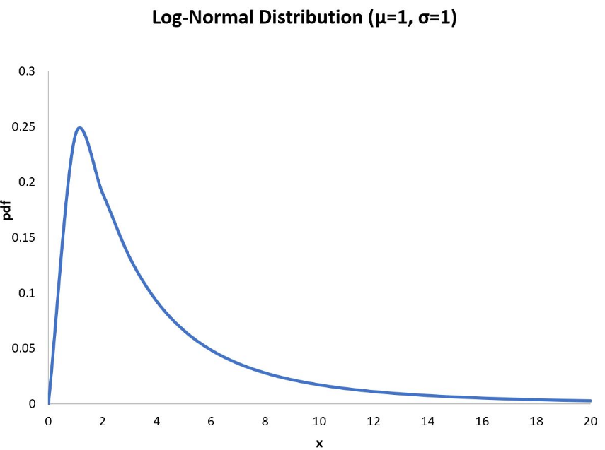
A Lognormal Distribution is commonly used in Discrete Event simulation to model the time to perform a task. It is right-skewed, which basically means it has a long tail. To put it in more understandable terms, it suggests that most activity times will be similar, but some will be longer, and some will be MUCH longer. This tends to capture activity times in patient pathways well.
12.1 A bit of background
Tip
The good news is that we will be using some prewritten code to specify our lognormal, and all we will need to know to do this is the mean (average) time for our activity, and the standard deviation (a measure of how much the times vary across the dataset that python can calculate for us if given a list of activity times).
However - it’s useful to have a bit more of an idea about what a lognormal is - so do have a read of the section below, but if you don’t quite get it just yet, don’t fret - just remember that lognormal is good for activity times in general, and the exponential distribution is good for inter-arrival times (the time between patients arriving).
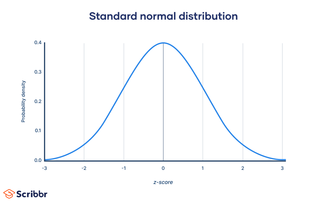
12.1.1 The normal distribution
A normal distribution is a bell shaped curve that is symmetrical. It is defined by two parameters : μ (Mu) and σ (Sigma), which represent the mean and standard deviation of the distribution. So it’s easy to plug in such values from our own data.
12.1.2 Logarithms
Before we proceed, let’s remind ourselves about something many of us learned at school (and then promptly forgot) : Logarithms.
Logarithms are basically the opposite of exponentials.
Effectively, lognormals relate to how many copies of one number multiply together to make another number.
How many 4s multiply together to make 64?
4 x 4 x 4 = 64 We had to multiply 3 copies of the number 4 to get 64.
This means that the logarithm is 3.
We’d write this as \[ Y = log_4(64) = 3 \]
12.1.3 Bringing it all together - lognormal distributions
How does this relate to the distribution?
Well, a Lognormal distribution is one in which the logarithm of the random variable we’re modelling is normally distributed.
This means that the the two parameters μ (Mu) and σ (Sigma) used to specify a Lognormal distribution do not represent the mean and standard deviation, unlike the normal distribution; rather, they represent what are known as the location and scale of the distribution respectively.
μ (Mu) and σ (Sigma) represent the mean and standard deviation once the data in the log normal distribution has been transformed using logarithms.
It’s easy to get the mean and standard deviation of our data.
If we used the Normal distribution, we could do that.
Warning
The Normal distribution often isn’t good for activity times - it allows negative values - activity distributions are rarely symmetrical - they’re more likely to be a bit ‘wonky’ (skewed), with just a few activities being much longer
The probalm is we can’t just give a Lognormal distribution the mean and standard deviation, because in a Lognormal distribution, the mean and standard deviation of our data is represented in the underlying normal distribution not the Lognormal distribution (remember, it’s the logarithms of the values that are normally distributed).
Tip
So what do we do?
We need to convert our mean and standard deviation values (that we get from our real world data) into Mu and Sigma for a Lognormal distribution.
This is the key bit you need to understand!
12.2 Code for the lognormal distribution
This code was written by Tom Monks.
We will add this into our model code.
Then we just need to make sure we have both a mean and standard deviation (SD) for activity times that we want to represent on Lognormal distributions
When we need to sample an activity time, we create an instance of the Lognormal class with our mean and SD, and call the sample method.
We are going to do this in the attend_clinic method of the Model class.
def attend_clinic(self, patient):
        # Nurse consultation activity
        start_q_nurse = self.env.now

        with self.nurse.request(priority=patient.priority) as req:
            yield req

            end_q_nurse = self.env.now

            patient.q_time_nurse = end_q_nurse - start_q_nurse

            if self.env.now > g.warm_up_period:
                self.results_df.at[patient.id, "Q Time Nurse"] = (
                    patient.q_time_nurse
                )

            ##NEW - we now use a lognormal distribution for the activity time,
            # so we create an instance of our Lognormal class with the mean
            # and standard deviations specified in g class, and then sample
            # from it (we do this in a single line of code here, much as we
            # did when sampling from the exponential distribution before).
            sampled_nurse_act_time = Lognormal(
                g.mean_n_consult_time, g.sd_n_consult_time).sample()

            yield self.env.timeout(sampled_nurse_act_time)
12.3 Additional distributions
In fact, there are many different distributions available.
The sim-tools package makes it easy to make use of them without having to write lots of classes yourself.
The source code for the package can be investigated in its Github Repository.
To install the package, run
pip install sim-toolsYou can then import a class with
from sim_tools.distributions import Exponentialreplacing Exponential with any of the supported distribution classes.
An overview of how to use the classes, and of the different distributions included, is embedded below: